1 Pledge

I’ll go dive about the history of pipes in R. Pipes have revolutionized the way we write R code, making it more readable and maintainable. But the story of pipes in R is richer than many realize. While most R users are already familiar with magrittr’s %>% or the native R |>, the journey of pipes in R spans multiple packages and years of implementations, each with unique features and use cases.

In this post, I’ll be chronological about what I explore in the history and variety of pipes available in R, from the pioneering days to modern implementations.

But the question still remains: How much did you really learn about pipes in R?

2 Brief Definition before starting

A pipe operator is a binary operator, just like +, that passes the output of one function as the input to the another expression. In R, it mimics Python’s method chaining:

R
Python

Without breaking into another line:

x |> f() |> g() |> h()

Breaking into next line:

x |> 
    f() |> 
    g() |> 
    h()

Without breaking into another line:

x.f().g().h()

Breaking into next line:

x \
    .f() \
    .g() \
    .h()
    
(
    x
      .f() 
      .g() 
      .h()
)

Note

In Python, you can’t break the code into another line, unless \ between the methods, or closing the expression with () is applied. As you can see, R is more forgiving and a lot better than Python, because it is only bounded in its class.

It lets you at least avoid creating intermediate variables and write code that reads from left to right — Usually, some documentation refers it as left-hand side (LHS) and right-hand side (RHS), respectively.

3 The Early Days: Pre-Pipe Workflows (≤2010)

Before pipes, the usual workflow in R relies on the following on nested function calls:

Nested function calls

round(mean(c(1, 2, 3, 4, 5)), 2)

[1] 3

This would be difficult to read and maintain once the function calls get deeper

round(mean(log(c(1, 2, 3, 4, 5))), 2)

[1] 0.96

Intermediate variables

Instead of a deep nested call

x = c(1, 2, 3, 4, 5)
log_x = log(x)
mu_x = mean(log_x)
mu_x_rounded = round(mu_x, 2)
mu_x_rounded

[1] 0.96

My problem with intermediate variables is that it is cluttered with temporary variables.

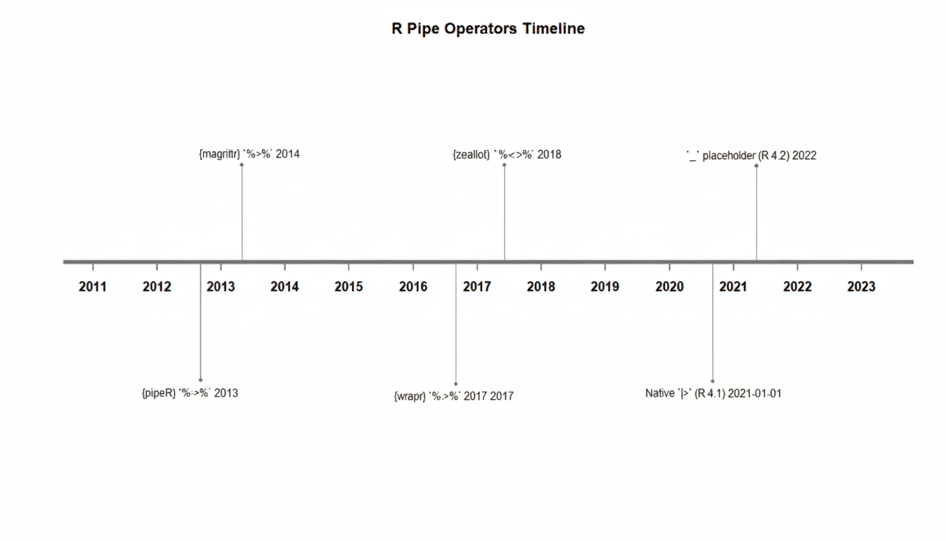
4 Timeline of R Pipes

Many of R developers in the past invented pipes, like many times. Let’s explore them chronologically.

See how pipes evolved from experimental packages to core R:

4.1 1. The {pipeR} Pioneer (2013)

The pipeR package by Kun Ren was one of the earliest pipe implementations in R, introducing the %>>% operator.

box::use(pipeR[`%>>%`])

1:10 %>>%
    mean() %>>%
    round(2)

[1] 5.5

Here’s the cool part:

Lambda expressions with parentheses:

1:10 %>>%
    (mean(.) * 2) %>>%
    round(2)

[1] 11

Side effects with continued piping:

set.seed(123)
rnorm(100) %>>%
    (~ plot(., main = "Random Normal Values")) %>>%  # Side effect
    mean() %>>%
    round(2)

[1] 0.09

Why it faded

It’s not like it vanished from the existence, more like it is superseded by magrittr and took over.

4.2 2. The Game Changer: {magrittr} Pipe (2014)

The magrittr package, created by Stefan Milton Bache and later maintained by Lionel Henry at Posit (formerly RStudio), became the most popular pipe implementation. It was inspired by F#’s pipe-forward operator and Unix pipes.

box::use(magrittr[`%>%`, `%<>%`, `%T>%`, `%$%`, `%!>%`])

c(1, 2, 3, 4, 5) %>%
    mean() %>%
    round(2)

[1] 3

Do you know? There are plenty pipe operators in magrittr package, consists of at least 5 operators. Here are the special features:

The %>% is magrittr’s standard and “lazy” pipe - it doesn’t evaluate arguments until needed, which can affect behavior with certain functions. Lazy evaluation means that the RHS is only computed when its value is required, which optimizes performance but can lead to surprises with side-effect-heavy code.

To understand better how %>% works, let’s give a demonstration by applying dot placeholder for non-first arguments:

mtcars %>%
    lm(mpg ~ cyl, data = .)


Call:
lm(formula = mpg ~ cyl, data = .)

Coefficients:
(Intercept)          cyl  
     37.885       -2.876

The dot (.) acts as a placeholder for the piped value, allowing it to be inserted into any argument position—not just the first. You can also apply multiple placeholders:

mtcars %>% 
    head(5) %>% 
    split(., .$cyl)

$`4`
            mpg cyl disp hp drat   wt  qsec vs am gear carb
Datsun 710 22.8   4  108 93 3.85 2.32 18.61  1  1    4    1

$`6`
                mpg cyl disp  hp drat    wt  qsec vs am gear carb
Mazda RX4      21.0   6  160 110 3.90 2.620 16.46  0  1    4    4
Mazda RX4 Wag  21.0   6  160 110 3.90 2.875 17.02  0  1    4    4
Hornet 4 Drive 21.4   6  258 110 3.08 3.215 19.44  1  0    3    1

$`8`
                   mpg cyl disp  hp drat   wt  qsec vs am gear carb
Hornet Sportabout 18.7   8  360 175 3.15 3.44 17.02  0  0    3    2

The %<>% operator is invoking reference semantics, where it pipes and assigns the result back to the original variable:

x = 1:5
x %<>% log() %>% sum()
x

[1] 4.787492

This is equivalent to x = x %>% log() %>% sum() but more concise. What happened here is we created a side-effect of x. Some pointed it out why it is a problem.

The %T>% “tee” pipe passes the left-hand side value forward, not the output of the right-hand side. Useful for side effects like plotting or printing, where you want to perform an action but continue with the original data:

set.seed(123)
rnorm(100) %T>% 
    plot(main = "Values before mean") %>% 
    mean() %>%
    round(2)

[1] 0.09

This should be the equivalent:

{
    set.seed(123)
    plot(rnorm(100), main = "Values before mean")
    round(mean(rnorm(100)), 2)
}

So, if you try the following:

1:5 %T>% 
    mean()

[1] 1 2 3 4 5

The %T>% operator discards the output of mean(1:5), and that’s because mean() doesn’t return a side-value effect.

By the way, the “tee” name comes from Unix’s tee command, which splits output streams.

The %$% “exposition” pipe exposes the names within the left-hand side object to the right-hand side expression:

mtcars %$%
    cor(mpg, cyl)

[1] -0.852162

This is equivalent to:

cor(mtcars$mpg, mtcars$cyl)

This is particularly useful with functions that don’t have a data argument.

Warning

Do not use %$% operator when LHS is not a a list or data frame with named elements.

The %!>% operator is the “eager” version of %>% that evaluates arguments immediately. This can matter for functions with non-standard evaluation:

# Standard (lazy) pipe
iris %>% 
    subset(Species == "setosa") %>% 
    head(3)

  Sepal.Length Sepal.Width Petal.Length Petal.Width Species
1          5.1         3.5          1.4         0.2  setosa
2          4.9         3.0          1.4         0.2  setosa
3          4.7         3.2          1.3         0.2  setosa

# Eager pipe (forces immediate evaluation)
iris %!>% 
    subset(Species == "setosa") %!>% 
    head(3)

  Sepal.Length Sepal.Width Petal.Length Petal.Width Species
1          5.1         3.5          1.4         0.2  setosa
2          4.9         3.0          1.4         0.2  setosa
3          4.7         3.2          1.3         0.2  setosa

In most cases, the difference is subtle, but it can matter for advanced programming.

To see the actual difference:

%!>%: cat(1) is immediately evaluated (it evaluates from left to right)

0 %!>% (\(x) { cat(1); x }) %!>% (\(x) cat(2))

%>%: Evaluates only cat(2) as the first result is never used

0 %>% (\(x) { cat(1); x }) %>% (\(x) cat(2))

Source: https://stackoverflow.com/questions/76326742/what-are-the-differences-and-use-cases-of-the-five-magrittr-pipes

4.3 3. The {wrapr} Dot Arrow (2017)

John Mount’s wrapr package provides the %.>% “dot arrow” pipe, a deliberate and explicit alternative to %>%.

box::use(wrapr[`%.>%`])

1:10 %.>%
    mean(.) %.>%
    round(., 2)

[1] 5.5

I don’t know much about this pipe, to be honest. As what I can see, this pipe requires the dot to always be explicit, which, for me, it’s so good that it can prevent some subtle bugs and makes code intentions clearer.

4.4 4. The Bizarro Pipe (Base R, ~2017)

I am not sure when this operator released, but there’s a pipe operator (not categorically) in base R: the “Bizarro pipe” (->.;), that works like %>% and %.>%. It’s not a formal operator but an emergent behavior from combining existing R syntax.

1:10 ->.; 
    mean(.) ->.; 
    round(., 2)

[1] 5.5

The Bizarro pipe works by:

Using right assignment -> to assign to . (this is done by typing - + > + .)
Ending each statement with ; to separate expressions
The next line uses . as input

It’s called “Bizarro” because it uses right-to-left assignment syntax (->) to create a left-to-right workflow.

However, it has disadvantages (talked in this Stackoverflow discussion):

Creates hidden side-effects (the persistent . variable)
Goes against R style guides (right assignment and semicolons are discouraged)
Can lead to subtle bugs if you forget to assign to . at some step
The . variable is hidden from ls() and IDE inspectors
It’s so pesky, it won’t auto-indent

Seriously, I won’t recommend Bizarro pipe at all. It is still a nice touch as a temporary replacement of %>% for chained R codes, and will not use it for production code.

4.5 5. The Native Pipe (R v4.1+, 2021)

In May 2021, R v4.1 introduced the native pipe operator |> (type | and >), bringing pipe functionality into base R without the need for external packages. This operator is the actual operator that was inspired by the pipe-forward operator in F# and the concept of Unix pipes.

c(1, 2, 3, 4, 5) |>
    mean() |>
    round(2)

[1] 3

This is too identical to %>% from magrittr with some obvious differences.

4.5.1 Common differences from `{magrittr}` pipe

The placeholder for |> is now applied in R v4.2 and above. For the syntax, it rather uses _, not ..

mtcars |>
    lm(mpg ~ cyl, data = _)


Call:
lm(formula = mpg ~ cyl, data = mtcars)

Coefficients:
(Intercept)          cyl  
     37.885       -2.876

The native pipe:

Is slightly faster (negligible in often cases, this matters for some cases like running for-loop)
Does not support the tee (%T>%), exposition (%$%), or assignment (%<>%) operators
Cannot be used with compound assignment
Is more strict about valid syntax

4.5.2 Performance comparison

The native pipe is clearly faster than the magrittr pipe because native pipe does not add more function calls within its implementation compared to the magrittr pipe.

bench::mark(
    "magrittr pipe" = replicate(10000, 1:100 %>% sum()), 
    "native R pipe" = replicate(10000, 1:100 |> sum())
)

# A tibble: 2 × 6
  expression         min   median `itr/sec` mem_alloc `gc/sec`
  <bch:expr>    <bch:tm> <bch:tm>     <dbl> <bch:byt>    <dbl>
1 magrittr pipe   49.6ms   53.5ms      18.7     375KB     65.4
2 native R pipe   11.6ms   13.8ms      64.7     369KB     27.7

4.5.3 Pipe-bind operator

After R v4.2, the pipe-bind operator => (type = + >), or a pipe-binding syntax, allows you to bind the result of the left-hand side (LHS) to a name within the right-hand side (RHS) expression.

This feature is, however, disabled by default. You may want to enable it by running the following:

Sys.setenv("_R_USE_PIPEBIND_" = TRUE)

Another options:

Place this command into .Renviron file (Hint: run usethis::edit_r_environ()):

_R_USE_PIPEBIND_=true

Run this in a command prompt or PowerShell

setx _R_USE_PIPEBIND_ true

If you are in Linux / macOS (bash / zsh):

export _R_USE_PIPEBIND_=true

Then restart R.

Here’s what it does:

mtcars |> 
    df => lm(mpg ~ wt, data = df)


Call:
lm(formula = mpg ~ wt, data = df)

Coefficients:
(Intercept)           wt  
     37.285       -5.344

mtcars |> 
    df => split(df, df$cyl) |> 
    lapply(\(df) lm(mpg ~ wt, data = df)) |> 
    vapply(\(mod) summary(mod)$r.squared, numeric(1))

        4         6         8 
0.5086326 0.4645102 0.4229655

The df name temporarily exists only inside that RHS expression — not in your global environment. I like this because this is more explicit than . in %>% operator. You can name the LHS result and refer to it directly inside the RHS expression anything you like.

4.6 Non-Pipe Alternatives

While the above are true pipe operators, it’s worth mentioning that some packages achieve similar left-to-right workflows through different mechanisms.

4.6.1 Chaining in {data.table} (2010)

data.table uses method chaining with [][] notation. It is NOT a pipe operator in a sense, but achieves a similar left-to-right flow. It behaves differently from the pipe operator — it chains operations within the same [.data.table method, and doesn’t pass values between functions, i.e. the use of placeholders.

Let’s look at the basic data.table example:

box::use(data.table[as.data.table, `:=`])

dt = as.data.table(mtcars)
dt[cyl == 8][order(-mpg)][, .(mpg, cyl, hp)][1:5]

     mpg   cyl    hp
   <num> <num> <num>
1:  19.2     8   175
2:  18.7     8   175
3:  17.3     8   180
4:  16.4     8   180
5:  15.8     8   264

Deeper method chaining in data.table with grouping and aggregation:

dt[, log_mpg := log(mpg)][,
    .(
        mpg_mean = mean(mpg, na.rm = TRUE), 
        log_mpg_mean = mean(log_mpg, na.rm = TRUE)
    ), by = cyl
][
    order(-mpg_mean, -log_mpg_mean)
]

     cyl mpg_mean log_mpg_mean
   <num>    <num>        <num>
1:     4 26.66364     3.270454
2:     6 19.74286     2.980439
3:     8 15.10000     2.700171

This is method chaining, not piping—the key difference is that pipes pass values between different functions, while data.table chains operations within the same [ method.

4.6.2 Multiple Assignment with {zeallot} (2018)

This is not exactly an operator that behaves like a pipe, where it passes LHS as an input for RHS, but I would like to point this one out. R lacks destructuring (also called “unpacking”) method, just like what you see in other languages, such as Python:

x, y = 0, 1

The zeallot allows destructuring assignment with %<-%. While not exactly a pipe operator to chain the commands, works well in pipe-like workflows.

box::use(zeallot[`%<-%`])

# Multiple assignment
c(a, b) %<-% c(1, 2)
c(a, b)

[1] 1 2

Destructuring with computations:

c(mean_val, sd_val, n) %<-% local ({
    set.seed(125)
    x = rnorm(100)
    c(mean(x), sd(x), length(x))
})

cat(glue::glue("Mean: {mean_val}, SD: {sd_val} , N: {n}"), "\n")

Mean: 0.100208694251594, SD: 1.06105719788861 , N: 100

Works with pipe workflows:

set.seed(123)
c(m, s) %<-% (rnorm(100) %>% { c(mean(.), sd(.)) })
c(m, s)

[1] 0.09040591 0.91281588

5 Acknowledgment

I would like to thank the r/rstats community for engaging my article about the pipes in R. I would like to thank u/guepier for pointing out the actual pipe history, where there’s actually a pipe that predates both pipeR and magrittr in this comment.

Special thanks to the developers of magrittr, pipeR, wrapr, and the R core team for introducing the native pipe operator.

6 Remarks and Resources

As you can see, it needs a lot to came up with lots of crufts and inventions, after years of invention. The native pipe came up later after the release of R v4.1 in May 2021, thanks to the popularization of magrittr and tidyverse. And that’s all I know about pipes in R.

Here are the additional resources:

1 Pledge

2 Brief Definition before starting

3 The Early Days: Pre-Pipe Workflows (≤2010)

4 Timeline of R Pipes

4.1 1. The {pipeR} Pioneer (2013)

4.2 2. The Game Changer: {magrittr} Pipe (2014)

4.3 3. The {wrapr} Dot Arrow (2017)

4.4 4. The Bizarro Pipe (Base R, ~2017)

4.5 5. The Native Pipe (R v4.1+, 2021)

4.5.1 Common differences from {magrittr} pipe

4.5.2 Performance comparison

4.5.3 Pipe-bind operator

4.6 Non-Pipe Alternatives

4.6.1 Chaining in {data.table} (2010)

4.6.2 Multiple Assignment with {zeallot} (2018)

5 Acknowledgment

6 Remarks and Resources

4.5.1 Common differences from `{magrittr}` pipe