Why SQL + R is an affable combo when I start learning SQL?

Learn mastering both — and how to make them work together seamlessly.
R
SQL
data-science
analytics
tidyverse
Author

Joshua Marie

Published

November 28, 2025

1 Introduction

I am already using R since 2018, and uses SQL since around 2022-2023. Way back in 2023, I am learning one of the most valuable feature in R, and that’s the ability to integrate R into other software. That’s because I only use softwares independently, i.e. R only, Python only, etc. This is how I first learn SQL, and I learn few frameworks that integrates R and SQL databases.

If you’ve spent any time in data science, I am sure you encountered language wars and such debates — there’s like hundreds or maybe thousands of blogs spread in the community comparing which languages is better or worse. I am not talking about that in this blog post, however, here’s the thing — it’s not really a versus situation. SQL and R are like peanut butter and jelly. Each is good on its own, but why not both? Flavorful.

Regardless, SQL excels at what databases do best: storing, organizing, and retrieving massive amounts of data with lightning speed. R, on the other hand, shines where creativity and complexity matter: statistical modeling, advanced visualizations, and transforming raw data into insights that actually mean something.

In this post, I’ll show you why combo-ing R and SQL isn’t just nice to have — it’s my stack. And more importantly, I’ll show you what I know how to make them work together so seamlessly you’ll wonder how you ever worked any other way.

2 Why Learn SQL Through R?

Before we dive into the technical details, let me explain why R is actually a fantastic environment for learning SQL:

  1. Immediate Feedback Loop

    When you’re learning SQL in a traditional database environment, you often need to set up servers, configure connections, and deal with authentication. With R, you can start writing queries in seconds and see results immediately in your familiar R environment.

  2. Best of Both Worlds

    You can write pure SQL when you want to practice, or use {dplyr} syntax and see the generated SQL. This dual approach accelerates learning because you can:

    • Write {dplyr} code and inspect the SQL it produces
    • Compare your hand-written SQL with {dbplyr}’s output
    • Gradually transition from {dplyr} comfort to SQL mastery
  3. Visualization Integration

    The moment you query data, you can pipe it directly into {ggplot2} or other R visualization tools. No export/import cycles, no switching between applications—just seamless analysis.

  4. Reproducible Workflows

    Everything lives in a script or R Markdown document. Your queries, analysis, and visualizations are all version-controlled and reproducible.

3 Tools and Packages

I can name few tools and packages on working with SQL databases in R, most especially when you just started. I don’t have any database in my own device, but did you know you can simulate databases? These are the tools and packages to start:

  1. {tidyverse} — Why this? This is a package that holds the complete set of tools in data science, and that includes working with databases. Speaking of which, this is a meta-package that also contains what we need: {dbplyr}, which also contains {DBI} package dependency.

  2. {box} — I already talked about this package in my previous blog posts. Please, take a look at them if you have some time:

  3. {dbplyr} — This is the magic translator. It converts your familiar {dplyr} code into SQL queries behind the scenes. You write R, it speaks SQL to the database. The best part? You can inspect the SQL it generates, which makes it a fantastic learning tool.

  4. {DBI} — Think of this as the universal adapter for database connections. It provides a consistent interface whether you’re connecting to SQLite, PostgreSQL, MySQL, or other databases. It handles the connection, sending queries, and fetching results.

  5. {RSQLite} — This is the R interface to SQLite databases. SQLite is perfect for learning because it’s lightweight, requires no server setup, and the entire database is just a single file on your computer.

Install them through this:

install.packages(c('tidyverse', 'box', 'RSQLite'))

Install them directly

pak::pak(c(
    'tidyverse', 
    'box', 
    'RSQLite'
))

When you preferred the development version

pak::pak(c(
    "tidyverse/tidyverse", 
    "klmr/box", 
    "r-dbi/RSQLite"
))

4 With existing database

I learn SQL thanks to SQLite. This is a language-agnostic library, written in C, that acts like a database while being lightweight. You can use it literally everywhere! It is also used to built into everywhere, it could be mobile phones and most computers.

Thanks to SQLite, I made a first move to learn SQL without installing heavy softwares, such as PostgreSQL and MySQL, just to learn SQL. Additionally, SQLite is an open-source, but not open for contribution (I believe this is designed for good purpose).

4.1 Why SQLite is Perfect for Learning

Here’s why SQLite is the ideal training ground:

  • No server required — It’s just a file on your computer
  • Zero configuration — No ports, users, or permissions to set up
  • Lightweight — Databases can be megabytes instead of gigabytes
  • Production-ready — Despite being “lite,” it’s used in production by major applications
  • SQL standard — You learn real SQL that transfers to other databases

In a positive sense, R and SQL is a great combo. Maybe R and SQL is not a great combo for software development as Python and SQL combo, R and SQL can make a place in data analysis instead. As long as you have {DBI} and {RSQLite} installed in your R, you can now make a first move on integrating R and SQL, and you’re good to go.

4.2 SQLite in R

Oh, you can definitely learn SQL and R at the same time, considering that SQLite is portable and lightweight. The only primary requirements are {DBI} and {RSQLite}. If you know how to write a query, you don’t need a compatible set of packages in {tidyverse} and {dbplyr}, otherwise, as long as you know how to use {tidyverse} packages, namely {dplyr}, {tidyr}, etc., you can use it instead.

Let me show you how to connect to a SQLite database and work with it:

box::use(
    DBI[dbConnect, dbWriteTable, dbDisconnect], 
    RSQLite[SQLite]
)


con = dbConnect(SQLite(), "first_database.sqlite")


df = data.frame(
    id = 1:5,
    name = c("Alice", "Bob", "Charlie", "Diana", "Eve"),
    age = c(25, 30, 35, 28, 42),
    city = c("New York", "London", "Tokyo", "Paris", "Sydney")
)


dbWriteTable(
    con, 
    "customers",
    df, 
    overwrite = TRUE
)
1
Create a connection (this creates the database file if it doesn’t exist)
2
Create some sample data
3
Write the data as a table to the database
  1. Create a connection (this creates the database file if it doesn’t exist)
  2. Create some sample data
  3. Write the data as a table to the database

What just happened?
We created a SQLite database file called first_database.sqlite in your working directory. Inside it, we created a table called customers with our sample data. If the file already exists, R simply connects to it.

4.3 Two Ways to Query: Pure SQL vs {dplyr}

Now comes the fun part—you can query this database in two different ways, and each has its benefits for learning.

Did you know that with {knitr}, you can write SQL code chunks directly in your R Markdown or Quarto documents? This is incredibly handy for mixing SQL queries with your data analysis in R.

```\{sql connection=con\}
SELECT name, age, city 
FROM customers 
WHERE age > 30
```

Kindly remove the \ when you copy the code chunk above.

Alright, I wrote the SQL code chunk above again here for your reference:

SELECT name, age, city 
FROM customers 
WHERE age > 30
2 records
name age city
Charlie 35 Tokyo
Eve 42 Sydney

Or you can store the query into a string, and send it via DBI::dbGetQuery(), placed in statement argument.

DBI::dbGetQuery(
    con, 
    "SELECT name, age, city \nFROM customers \nWHERE age > 30"
)
     name age   city
1 Charlie  35  Tokyo
2     Eve  42 Sydney

Why this matters for learning:
You’re writing actual SQL. No training wheels. This builds muscle memory for SQL syntax and helps you think in terms of SQL operations: SELECT, FROM, WHERE, JOIN, GROUP BY, etc.

Nothing can make it so easy to work with databases using a familiar syntax with {dplyr}. Yes, with {dbplyr}, you can use {dplyr} functions to interact with your database tables as if they were regular data frames in R. Here’s how you can perform the same query using {dplyr}:

box::use(
    dplyr[filter, select, tbl, collect, show_query]
)

customers_tbl = tbl(con, "customers")

out = customers_tbl |> 
    filter(age > 30) |> 
    select(name, age, city)

out |> collect()
# A tibble: 2 × 3
  name      age city  
  <chr>   <dbl> <chr> 
1 Charlie    35 Tokyo 
2 Eve        42 Sydney

The magic behind this:

When you use {dplyr} verbs on a database table, {dbplyr} doesn’t immediately execute anything. It’s lazy! It builds up the query and only executes it when you call collect(). This is efficient because:

  • You can chain many operations without multiple round-trips to the database
  • Only the final result set gets pulled into R memory
  • The heavy computation happens in the database where it’s optimized

See the generated SQL:

How about getting the SQL query generated by {dbplyr}? You can use the show_query() function to see the SQL that {dbplyr} generates for your {dplyr} code:

out |> 
    show_query()
<SQL>
SELECT `name`, `age`, `city`
FROM `customers`
WHERE (`age` > 30.0)

Easy, right? If you know R already, treat it as your SQL teacher! Write familiar {dplyr} code, then check the SQL translation. Over time, you’ll start to intuitively understand how filter() becomes WHERE, how select() becomes SELECT, and how more complex operations translate to SQL.

4.4 Working with Query Results

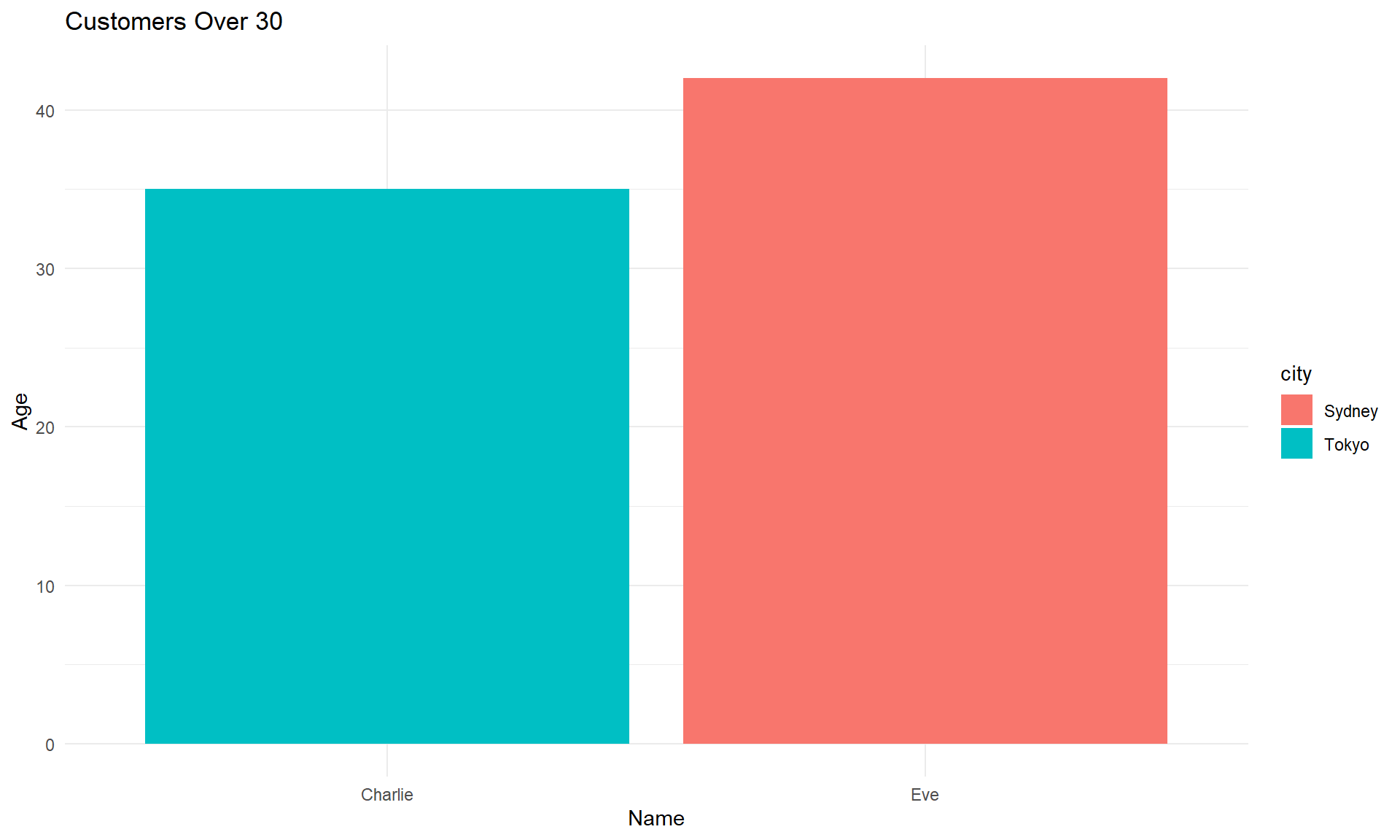
Once you have query results, you can treat them like any R data frame:

box::use(
    ggplot2[ggplot, aes, geom_col, theme_minimal, labs]
)


result_data = collect(out)


result_data |>  
    ggplot(aes(x = name, y = age, fill = city)) +
    geom_col() +
    theme_minimal() +
    labs(
        title = "Customers Over 30",
        x = "Name",
        y = "Age"
    )
1
Retrieve the data
2
Now you can analyze it with R

  1. Retrieve the data
  2. Now you can analyze it with R

This is where the R + SQL combination really shines. You use SQL’s efficiency to get exactly the data you need, then R’s rich ecosystem for analysis and visualization.

4.5 Database Hygiene

Always remember to close your database connections once you’re done:

dbDisconnect(con)

This releases resources and ensures your database file isn’t locked. In practice, connections are also closed automatically when your R session ends, but it’s good practice to do it explicitly.

5 Learning SQL in R without a server

But I know some of you wants to know what it looks like to use the existing database and then call it in R.

I literally said in the introduction that you can simulate — I have another different meaning:

  • Use simulate_* family functions in {dbplyr} package. These functions allow you to create in-memory database tables that mimic real database behavior without needing an actual database server. This is perfect for learning and testing SQL queries in R.

5.1 What Are Simulated Connections?

Simulated connections create an in-memory representation of how different database systems handle SQL. This means you can:

  • See how your {dplyr} code translates to different SQL dialects
  • Learn SQL without any database installation
  • Test queries before running them on production databases
  • Understand the quirks of different database systems

5.2 Demonstration: Simulating Microsoft SQL Server

First, let me show you how it looks like to connect to a database, i.e. SQLite in this case, and work with it. Try imagine you have a SQL server, and you want to connect to it using R. Use simulate_mssql() function to simulate a Microsoft SQL Server database connection:

box::use(
    dbplyr[simulate_mssql, tbl_lazy]
)

con_sim = simulate_mssql()
customers_sim = tbl_lazy(df, con_sim)

customers_sim |>
    select(name, age, city) |>
    filter(age > 30)
1
Create a simulated MS SQL Server connection
2
Create a (local) lazy table from our data frame
3
Build a query
<SQL>
SELECT `name`, `age`, `city`
FROM `df`
WHERE (`age` > 30.0)
  1. Create a simulated MS SQL Server connection
  2. Create a (local) lazy table from our data frame
  3. Build a query

We are performing a pure lazy evaluation in this step. Which means, we are not returning any information in the table and in the query process, we only generate the SQL code.

5.3 Comparing SQL Dialects

The only issue when learning SQL with R in the past is when I found out that different databases have different SQL dialects. Let’s compare how PostgreSQL and Microsoft SQL Server handle the same query:

Let’s import a bit first:

box::use(
    dplyr[
        keep_when = filter, arrange, desc, show_query, 
        summarise, mutate, relocate
    ], 
    tidyr[
        long = pivot_longer
    ], 
    dbplyr[simulate_postgres, simulate_mssql], 
    magrittr[`%>%`]
)
1
This is totally optional, you still can use |> base R pipes, after all.

5.3.1 PostgreSQL version

con_postgres = simulate_postgres()
mtcars_postgres = tbl_lazy(mtcars, con_postgres)

mtcars_postgres %>% 
    filter(cyl == 6) %>% 
    mutate(
        hp_per_cyl = hp / cyl,
        efficiency = mpg / disp
    ) %>% 
    select(mpg, disp, hp, hp_per_cyl, efficiency, everything()) %>% 
    summarise(
        across(
            c(mpg, hp_per_cyl, efficiency), 
            list(
                mu = \(x) mean(x, na.rm = TRUE), 
                sigma = \(x) sd(x, na.rm = TRUE)
            ), 
            .names = "{.col}..{.fn}"
        ),
        n = n()
    ) %>% 
    long(
        cols = contains(c("mu", "sigma")), 
        names_sep = "\\..", 
        names_to = c("Variable", "Stat"), 
        values_to = "Est"
    )
Click to view generated SQL code
<SQL>
SELECT `n`, 'mpg' AS `Variable`, 'mu' AS `Stat`, `mpg..mu` AS `Est`
FROM (
  SELECT
    AVG(`mpg`) AS `mpg..mu`,
    STDDEV_SAMP(`mpg`) AS `mpg..sigma`,
    AVG(`hp_per_cyl`) AS `hp_per_cyl..mu`,
    STDDEV_SAMP(`hp_per_cyl`) AS `hp_per_cyl..sigma`,
    AVG(`efficiency`) AS `efficiency..mu`,
    STDDEV_SAMP(`efficiency`) AS `efficiency..sigma`,
    COUNT(*) AS `n`
  FROM (
    SELECT
      `mpg`,
      `disp`,
      `hp`,
      `hp` / `cyl` AS `hp_per_cyl`,
      `mpg` / `disp` AS `efficiency`,
      `cyl`,
      `drat`,
      `wt`,
      `qsec`,
      `vs`,
      `am`,
      `gear`,
      `carb`
    FROM `df`
    WHERE (`cyl` = 6.0)
  ) AS `q01`
) AS `q01`
UNION ALL

SELECT
  `n`,
  'hp_per_cyl' AS `Variable`,
  'mu' AS `Stat`,
  `hp_per_cyl..mu` AS `Est`
FROM (
  SELECT
    AVG(`mpg`) AS `mpg..mu`,
    STDDEV_SAMP(`mpg`) AS `mpg..sigma`,
    AVG(`hp_per_cyl`) AS `hp_per_cyl..mu`,
    STDDEV_SAMP(`hp_per_cyl`) AS `hp_per_cyl..sigma`,
    AVG(`efficiency`) AS `efficiency..mu`,
    STDDEV_SAMP(`efficiency`) AS `efficiency..sigma`,
    COUNT(*) AS `n`
  FROM (
    SELECT
      `mpg`,
      `disp`,
      `hp`,
      `hp` / `cyl` AS `hp_per_cyl`,
      `mpg` / `disp` AS `efficiency`,
      `cyl`,
      `drat`,
      `wt`,
      `qsec`,
      `vs`,
      `am`,
      `gear`,
      `carb`
    FROM `df`
    WHERE (`cyl` = 6.0)
  ) AS `q01`
) AS `q01`
UNION ALL

SELECT
  `n`,
  'efficiency' AS `Variable`,
  'mu' AS `Stat`,
  `efficiency..mu` AS `Est`
FROM (
  SELECT
    AVG(`mpg`) AS `mpg..mu`,
    STDDEV_SAMP(`mpg`) AS `mpg..sigma`,
    AVG(`hp_per_cyl`) AS `hp_per_cyl..mu`,
    STDDEV_SAMP(`hp_per_cyl`) AS `hp_per_cyl..sigma`,
    AVG(`efficiency`) AS `efficiency..mu`,
    STDDEV_SAMP(`efficiency`) AS `efficiency..sigma`,
    COUNT(*) AS `n`
  FROM (
    SELECT
      `mpg`,
      `disp`,
      `hp`,
      `hp` / `cyl` AS `hp_per_cyl`,
      `mpg` / `disp` AS `efficiency`,
      `cyl`,
      `drat`,
      `wt`,
      `qsec`,
      `vs`,
      `am`,
      `gear`,
      `carb`
    FROM `df`
    WHERE (`cyl` = 6.0)
  ) AS `q01`
) AS `q01`

UNION ALL

SELECT `n`, 'mpg' AS `Variable`, 'sigma' AS `Stat`, `mpg..sigma` AS `Est`
FROM (
  SELECT
    AVG(`mpg`) AS `mpg..mu`,
    STDDEV_SAMP(`mpg`) AS `mpg..sigma`,
    AVG(`hp_per_cyl`) AS `hp_per_cyl..mu`,
    STDDEV_SAMP(`hp_per_cyl`) AS `hp_per_cyl..sigma`,
    AVG(`efficiency`) AS `efficiency..mu`,
    STDDEV_SAMP(`efficiency`) AS `efficiency..sigma`,
    COUNT(*) AS `n`
  FROM (
    SELECT
      `mpg`,
      `disp`,
      `hp`,
      `hp` / `cyl` AS `hp_per_cyl`,
      `mpg` / `disp` AS `efficiency`,
      `cyl`,
      `drat`,
      `wt`,
      `qsec`,
      `vs`,
      `am`,
      `gear`,
      `carb`
    FROM `df`
    WHERE (`cyl` = 6.0)
  ) AS `q01`
) AS `q01`

UNION ALL

SELECT
  `n`,
  'hp_per_cyl' AS `Variable`,
  'sigma' AS `Stat`,
  `hp_per_cyl..sigma` AS `Est`
FROM (
  SELECT
    AVG(`mpg`) AS `mpg..mu`,
    STDDEV_SAMP(`mpg`) AS `mpg..sigma`,
    AVG(`hp_per_cyl`) AS `hp_per_cyl..mu`,
    STDDEV_SAMP(`hp_per_cyl`) AS `hp_per_cyl..sigma`,
    AVG(`efficiency`) AS `efficiency..mu`,
    STDDEV_SAMP(`efficiency`) AS `efficiency..sigma`,
    COUNT(*) AS `n`
  FROM (
    SELECT
      `mpg`,
      `disp`,
      `hp`,
      `hp` / `cyl` AS `hp_per_cyl`,
      `mpg` / `disp` AS `efficiency`,
      `cyl`,
      `drat`,
      `wt`,
      `qsec`,
      `vs`,
      `am`,
      `gear`,
      `carb`
    FROM `df`
    WHERE (`cyl` = 6.0)
  ) AS `q01`
) AS `q01`

UNION ALL

SELECT
  `n`,
  'efficiency' AS `Variable`,
  'sigma' AS `Stat`,
  `efficiency..sigma` AS `Est`
FROM (
  SELECT
    AVG(`mpg`) AS `mpg..mu`,
    STDDEV_SAMP(`mpg`) AS `mpg..sigma`,
    AVG(`hp_per_cyl`) AS `hp_per_cyl..mu`,
    STDDEV_SAMP(`hp_per_cyl`) AS `hp_per_cyl..sigma`,
    AVG(`efficiency`) AS `efficiency..mu`,
    STDDEV_SAMP(`efficiency`) AS `efficiency..sigma`,
    COUNT(*) AS `n`
  FROM (
    SELECT
      `mpg`,
      `disp`,
      `hp`,
      `hp` / `cyl` AS `hp_per_cyl`,
      `mpg` / `disp` AS `efficiency`,
      `cyl`,
      `drat`,
      `wt`,
      `qsec`,
      `vs`,
      `am`,
      `gear`,
      `carb`
    FROM `df`
    WHERE (`cyl` = 6.0)
  ) AS `q01`
) AS `q01`

5.3.2 Microsoft SQL Server version

con_mssql = simulate_mssql()
mtcars_mssql = tbl_lazy(mtcars, con_mssql)

mtcars_mssql %>% 
    filter(cyl == 6) %>% 
    mutate(
        hp_per_cyl = hp / cyl,
        efficiency = mpg / disp
    ) %>% 
    select(mpg, disp, hp, hp_per_cyl, efficiency, everything()) %>% 
    summarise(
        across(
            c(mpg, hp_per_cyl, efficiency), 
            list(
                mu = \(x) mean(x, na.rm = TRUE), 
                sigma = \(x) sd(x, na.rm = TRUE)
            ), 
            .names = "{.col}..{.fn}"
        ),
        n = n()
    ) %>% 
    long(
        cols = contains(c("mu", "sigma")), 
        names_sep = "\\..", 
        names_to = c("Variable", "Stat"), 
        values_to = "Est"
    )
Click to view generated SQL code
<SQL>
SELECT `n`, 'mpg' AS `Variable`, 'mu' AS `Stat`, `mpg..mu` AS `Est`
FROM (
  SELECT
    AVG(`mpg`) AS `mpg..mu`,
    STDEV(`mpg`) AS `mpg..sigma`,
    AVG(`hp_per_cyl`) AS `hp_per_cyl..mu`,
    STDEV(`hp_per_cyl`) AS `hp_per_cyl..sigma`,
    AVG(`efficiency`) AS `efficiency..mu`,
    STDEV(`efficiency`) AS `efficiency..sigma`,
    COUNT_BIG(*) AS `n`
  FROM (
    SELECT
      `mpg`,
      `disp`,
      `hp`,
      `hp` / `cyl` AS `hp_per_cyl`,
      `mpg` / `disp` AS `efficiency`,
      `cyl`,
      `drat`,
      `wt`,
      `qsec`,
      `vs`,
      `am`,
      `gear`,
      `carb`
    FROM `df`
    WHERE (`cyl` = 6.0)
  ) AS `q01`
) AS `q01`

UNION ALL

SELECT
  `n`,
  'hp_per_cyl' AS `Variable`,
  'mu' AS `Stat`,
  `hp_per_cyl..mu` AS `Est`
FROM (
  SELECT
    AVG(`mpg`) AS `mpg..mu`,
    STDEV(`mpg`) AS `mpg..sigma`,
    AVG(`hp_per_cyl`) AS `hp_per_cyl..mu`,
    STDEV(`hp_per_cyl`) AS `hp_per_cyl..sigma`,
    AVG(`efficiency`) AS `efficiency..mu`,
    STDEV(`efficiency`) AS `efficiency..sigma`,
    COUNT_BIG(*) AS `n`
  FROM (
    SELECT
      `mpg`,
      `disp`,
      `hp`,
      `hp` / `cyl` AS `hp_per_cyl`,
      `mpg` / `disp` AS `efficiency`,
      `cyl`,
      `drat`,
      `wt`,
      `qsec`,
      `vs`,
      `am`,
      `gear`,
      `carb`
    FROM `df`
    WHERE (`cyl` = 6.0)
  ) AS `q01`
) AS `q01`

UNION ALL

SELECT
  `n`,
  'efficiency' AS `Variable`,
  'mu' AS `Stat`,
  `efficiency..mu` AS `Est`
FROM (
  SELECT
    AVG(`mpg`) AS `mpg..mu`,
    STDEV(`mpg`) AS `mpg..sigma`,
    AVG(`hp_per_cyl`) AS `hp_per_cyl..mu`,
    STDEV(`hp_per_cyl`) AS `hp_per_cyl..sigma`,
    AVG(`efficiency`) AS `efficiency..mu`,
    STDEV(`efficiency`) AS `efficiency..sigma`,
    COUNT_BIG(*) AS `n`
  FROM (
    SELECT
      `mpg`,
      `disp`,
      `hp`,
      `hp` / `cyl` AS `hp_per_cyl`,
      `mpg` / `disp` AS `efficiency`,
      `cyl`,
      `drat`,
      `wt`,
      `qsec`,
      `vs`,
      `am`,
      `gear`,
      `carb`
    FROM `df`
    WHERE (`cyl` = 6.0)
  ) AS `q01`
) AS `q01`

UNION ALL

SELECT `n`, 'mpg' AS `Variable`, 'sigma' AS `Stat`, `mpg..sigma` AS `Est`
FROM (
  SELECT
    AVG(`mpg`) AS `mpg..mu`,
    STDEV(`mpg`) AS `mpg..sigma`,
    AVG(`hp_per_cyl`) AS `hp_per_cyl..mu`,
    STDEV(`hp_per_cyl`) AS `hp_per_cyl..sigma`,
    AVG(`efficiency`) AS `efficiency..mu`,
    STDEV(`efficiency`) AS `efficiency..sigma`,
    COUNT_BIG(*) AS `n`
  FROM (
    SELECT
      `mpg`,
      `disp`,
      `hp`,
      `hp` / `cyl` AS `hp_per_cyl`,
      `mpg` / `disp` AS `efficiency`,
      `cyl`,
      `drat`,
      `wt`,
      `qsec`,
      `vs`,
      `am`,
      `gear`,
      `carb`
    FROM `df`
    WHERE (`cyl` = 6.0)
  ) AS `q01`
) AS `q01`

UNION ALL

SELECT
  `n`,
  'hp_per_cyl' AS `Variable`,
  'sigma' AS `Stat`,
  `hp_per_cyl..sigma` AS `Est`
FROM (
  SELECT
    AVG(`mpg`) AS `mpg..mu`,
    STDEV(`mpg`) AS `mpg..sigma`,
    AVG(`hp_per_cyl`) AS `hp_per_cyl..mu`,
    STDEV(`hp_per_cyl`) AS `hp_per_cyl..sigma`,
    AVG(`efficiency`) AS `efficiency..mu`,
    STDEV(`efficiency`) AS `efficiency..sigma`,
    COUNT_BIG(*) AS `n`
  FROM (
    SELECT
      `mpg`,
      `disp`,
      `hp`,
      `hp` / `cyl` AS `hp_per_cyl`,
      `mpg` / `disp` AS `efficiency`,
      `cyl`,
      `drat`,
      `wt`,
      `qsec`,
      `vs`,
      `am`,
      `gear`,
      `carb`
    FROM `df`
    WHERE (`cyl` = 6.0)
  ) AS `q01`
) AS `q01`

UNION ALL

SELECT
  `n`,
  'efficiency' AS `Variable`,
  'sigma' AS `Stat`,
  `efficiency..sigma` AS `Est`
FROM (
  SELECT
    AVG(`mpg`) AS `mpg..mu`,
    STDEV(`mpg`) AS `mpg..sigma`,
    AVG(`hp_per_cyl`) AS `hp_per_cyl..mu`,
    STDEV(`hp_per_cyl`) AS `hp_per_cyl..sigma`,
    AVG(`efficiency`) AS `efficiency..mu`,
    STDEV(`efficiency`) AS `efficiency..sigma`,
    COUNT_BIG(*) AS `n`
  FROM (
    SELECT
      `mpg`,
      `disp`,
      `hp`,
      `hp` / `cyl` AS `hp_per_cyl`,
      `mpg` / `disp` AS `efficiency`,
      `cyl`,
      `drat`,
      `wt`,
      `qsec`,
      `vs`,
      `am`,
      `gear`,
      `carb`
    FROM `df`
    WHERE (`cyl` = 6.0)
  ) AS `q01`
) AS `q01`

5.4 When to Use Simulated Connections

Simulated connections are perfect for:

  • Learning: Practice SQL translation without database setup
  • Development: Test query logic before connecting to real databases
  • Documentation: Show how queries work across different systems
  • Teaching: Demonstrate SQL concepts without infrastructure requirements

6 Common Pitfalls and How to Avoid Them

Some are based on my experience, so some of the list can be opinionated.

6.1 1. Collecting Too Early

The problem in R can be overdramatic with large amounts of data when read and processed into memory. Unnecessarily bringing entire tables into R memory creates performance bottlenecks and can even crash your R session when datasets exceed available RAM.

Chain operations and collect only when needed. Let the database do the heavy lifting with filtering, aggregating, and joining before bringing results into R.

6.2 2. Not Checking Query Plans

Slow queries are often the result of poor optimization, but many users never investigate why their queries take so long. Without examining the query plan, you’re flying blind—unable to identify bottlenecks, missing indexes, or inefficient joins.

Use explain() to understand query execution. This reveals how the database processes your query and highlights optimization opportunities.

6.3 3. Forgetting Database Differences

SQL dialects vary between database systems, and code that runs perfectly in SQLite might fail spectacularly in PostgreSQL or MySQL. These differences range from subtle syntax variations to completely different function names and behaviors.

Test with simulated connections and understand dialect differences. Use {dbplyr}’s simulate_*() functions to preview how queries translate across databases before deploying to production systems.

6.4 4. Ignoring Indexes

Queries that scan entire tables are a common performance killer, especially as datasets grow. Without proper indexes, your database must examine every single row to find matches, turning what should be millisecond queries into multi-second ordeals.

Learn about indexes and how to create them for frequently queried columns. Understand which columns benefit from indexing and how composite indexes can optimize complex queries.

6.5 5. Not Parameterizing Queries

Building queries with string concatenation isn’t just inelegant—it’s dangerous. This practice opens your code to SQL injection attacks, where malicious input can execute arbitrary database commands, potentially exposing or destroying data.

Use parameterized queries with DBI::dbBind() or stick with {dplyr} operations, which handle parameterization automatically. Never concatenate user input directly into SQL strings.

7 Conclusion

SQL and R aren’t competitors — they’re collaborators. SQL is your data retrieval expert, getting you exactly the data you need with incredible efficiency. R is your analysis specialist, turning that data into insights, models, and visualizations. I can guarantee you that learning SQL through R is that you’re never starting from zero. Your existing R knowledge accelerates SQL mastery. The familiar {dplyr} syntax becomes your bridge to SQL fluency. And the ability to seamlessly move from database queries to statistical analysis to stunning visualizations—all in one environment—is genuinely powerful.

The data-driven professionals who thrive are those who can speak both languages fluently. They use SQL to ask databases the right questions and R to find the answers that matter. They understand when to leverage database optimization and when to bring data into R for complex transformations.

The journey from R user to R + SQL expert isn’t just about learning syntax—it’s about becoming someone who can efficiently bridge data storage and data science, who understands both the “how” of data retrieval and the “why” of data analysis.

So don’t pick sides. Master both. Your future self (and would be your future employers) will thank you.